Tutorial
This tutorial shows the current aleathor workflow: build or load a CSG model, query it, plot slices, trace rays, and export results. The API is still alpha, so conversion and large-model workflows should be validated against your transport code before production use.
All examples assume:
import aleathor as ath
1. Build A Small Model
You can start from an existing MCNP/OpenMC file, but a small Python-built model is the clearest first example:
model = ath.Model("Sphere in box")

sphere = ath.Sphere(0, 0, 0, radius=5.0)
box = ath.RPP(-10, 10, -10, 10, -10, 10)

fuel = -sphere
moderator = -box & +sphere

model.add_cell(fuel, material=1, density=10.5, name="fuel")
model.add_cell(moderator, material=2, density=1.0, name="moderator")

print(model)
In Python, density is a positive magnitude. By default it is treated as mass density (density_unit="g/cm3"), which is written with MCNP's negative density syntax on export. Use density_unit="atoms/b-cm" for atom density.
2. Load Existing Geometry
For real work, the usual entry point is an existing geometry file:
model = ath.load("geometry.inp")       # MCNP by default
model = ath.load("geometry.xml")       # OpenMC from .xml extension
You can also be explicit:
model = ath.read_mcnp("geometry.inp")
model = ath.read_openmc("geometry.xml")
Or load MCNP text directly:
mcnp_input = """1 1 -10.0 -1
2 0 1

1 SO 5.0

"""
model = ath.read_mcnp_string(mcnp_input)
The returned Model is ready for queries. Query acceleration is prepared automatically when needed.
3. Query Points
Use cell_at() for the normal "what is here?" question:
cell = model.cell_at(0.0, 0.0, 0.0)
if cell is None:
    print("Point is in void or undefined space")
else:
    print(f"Cell {cell.id}, material {cell.material}, density {cell.density}")
Use cell_path_at() only when debugging nested universes and FILLs:
for cell in model.cell_path_at(0.0, 0.0, 0.0):
    print(f"depth={cell.depth}: cell={cell.id}, universe={cell.universe}")
In a flat model this is usually a one-cell list. In a nested model it shows the path from the outer container to the terminal cell.
If you already know the cell ID:
cell = model[1]              # Same as model.get_cell(1)
print(cell.material)
print(cell.bounds)
4. Filter Cells
model.cells is a CellCollection:
for cell in model.cells:
    print(cell.id, cell.material, cell.universe)

fuel_cells = model.cells.by_material(1)
root_cells = model.cells.by_universe(0)
filled_cells = model.cells.by_fill()

dense = model.cells.filter(lambda c: c.density > 5.0)

print(model.cells.ids())
print(model.cells.materials())
print(model.cells.universes())
Prefer model.cells for user code; it returns Cell views rather than backend indices.
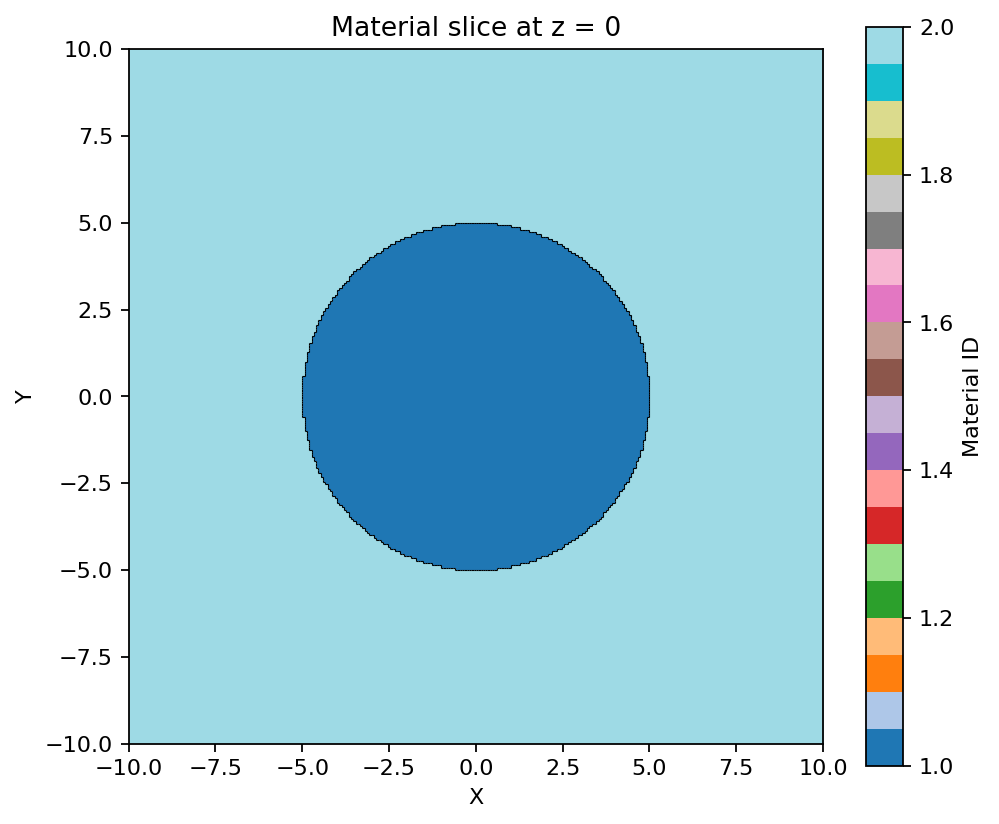
5. Plot Slices
Plotting is installed with aleathor and uses matplotlib/numpy.
model.plot(z=0, bounds=(-10, 10, -10, 10))
model.plot(y=0, bounds=(-10, 10, -10, 10))
model.plot(x=0, bounds=(-10, 10, -10, 10))
Useful options:
model.plot(z=0, bounds=(-10, 10, -10, 10), by_material=True)

model.plot(
    z=0,
    bounds=(-10, 10, -10, 10),
    by_material=True,
    show_colorbar=True,
    contour_by="cell",
)

model.plot_views(bounds=(-10, 10, -10, 10, -10, 10), save="views.png")
For raw slice data:
grid = model.slice.grid(
    axis="z",
    value=0,
    bounds=(-10, 10, -10, 10),
    resolution=(200, 200),
)

cell_ids = grid["cell_ids"]
material_ids = grid["material_ids"]
For arbitrary planes, use origin, normal, and optionally up:
model.plot(
    origin=(0, 0, 0),
    normal=(1, 1, 0),
    up=(0, 0, 1),
    bounds=(-10, 10, -10, 10),
)
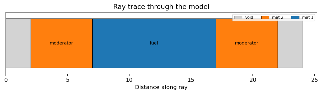
6. Trace Rays
Trace from an origin along a direction:
trace = model.trace(
    origin=(-10, 0, 0),
    direction=(1, 0, 0),
    max_distance=20,
)

for seg in trace:
    if seg.cell is None:
        print(f"void: {seg.length:.3f}")
    else:
        print(f"cell {seg.cell.id}: material {seg.material}, length {seg.length:.3f}")
Or trace between two points:
trace = model.trace(start=(-10, 0, 0), end=(10, 0, 0))
Analyze the result:
print(trace.path_length())              # Total non-void path length
print(trace.path_length(material=1))    # Path through material 1
print(trace.materials_hit())
print(trace.cells_hit())
For large models, cell_aware=True can be faster:
trace = model.trace(start=(-10, 0, 0), end=(10, 0, 0), cell_aware=True)
7. Mutate Cells
Cells are C-backed views. Property setters update the C backend directly:
cell = model[1]
cell.material = 3
cell.density = 7.8
cell.density_unit = "g/cm3"
cell.name = "steel"
You can also update through the model:
model.update_cell(1, material=3, density=7.8)
FILL can be changed through the Cell view:
cell.fill = 5
8. Universes And FILLs
Define reusable geometry in one universe, then fill a container cell with that universe:
pin = ath.Model("Pin")

fuel = ath.Sphere(0, 0, 0, radius=0.4)
clad = ath.ZCylinder(0, 0, radius=0.5)
box = ath.RPP(-1, 1, -1, 1, -1, 1)

pin.add_cell(-fuel, material=1, density=10.0, universe=1, name="fuel")
pin.add_cell(-clad & +fuel, material=2, density=6.5, universe=1, name="clad")
pin.add_cell(-box, fill=1, universe=0, name="pin container")

print(pin.cell_at(0, 0, 0))
print([c.id for c in pin.cell_path_at(0, 0, 0)])
cell_at() returns the terminal cell. cell_path_at() shows the parent/container cells as well.
9. Export
Use save() and let aleathor choose the format from the extension:
model.save("geometry.inp")      # MCNP
model.save("geometry.xml")      # OpenMC
model.save("geometry.serp")     # Serpent
MCNP text can also be generated as a string:
mcnp_text = model.to_mcnp_string()
Format conversion uses the same load/save API, but remains alpha:
model = ath.load("input.inp")
model.save("geometry.xml")
Always inspect and validate converted output before using it for production transport runs.
The explicit methods export_mcnp(), export_openmc(), and export_serpent() are also available when you do not want extension-based detection.
10. Validation
Overlap search is sampling-based:
for c1, c2 in model.analysis.find_overlaps():
    print(f"Possible overlap: {c1.id}, {c2.id}")
Slice-level checks can mark overlap or undefined pixels:
grid = model.slice.grid(
    axis="z",
    value=0,
    bounds=(-10, 10, -10, 10),
    resolution=(200, 200),
    detect_errors=True,
)

errors = model.slice.check_overlaps(grid)
11. Mesh Sampling And Export
Sample a structured mesh without writing a file:
mesh = model.mesh.sample(
    nx=50,
    ny=50,
    nz=50,
    bounds=(-10, 10, -10, 10, -10, 10),
)

materials = mesh["material_ids"]
cells = mesh["cell_ids"]
Export to Gmsh or VTK:
model.mesh.export(
    "geometry.msh",
    nx=50,
    ny=50,
    nz=50,
    bounds=(-10, 10, -10, 10, -10, 10),
)

model.mesh.export(
    "geometry.vtk",
    nx=50,
    ny=50,
    nz=50,
    bounds=(-10, 10, -10, 10, -10, 10),
    format="vtk",
)
12. Advanced Operations
These are useful once you are working on larger or imported models:
stats = model.repair.simplify()
model.repair.expand_macrobodies()
model.repair.tighten_bboxes(tolerance=1.0)
simplify() rewrites CSG trees; expand_macrobodies() turns MCNP macrobodies into primitive surfaces where supported; tighten_bboxes() improves cell bounding boxes used by spatial queries.
13. Logging
ath.enable_logging()
ath.set_log_level(ath.LOG_DEBUG)
ath.disable_logging()
Next Steps
- Read Concepts for surfaces, sense, regions, cells, and universes.
- Read API Reference for the complete public API.
- Read Current Status for alpha-stage caveats.